Multivariate analysis vs multiple univariate analyses

I once read a paper where the author said that shape’s a multidimensional and multivariate character. That let me thinking for months on the difference between these two terms. The next summer, during an oral presentation, a different scientist repeated that same sentence, this time explaining that shape’s a multidimensional character due to the number of variables that are used to describe it and a multivariate character due to the statistical treatment this character must receive to be analysed. Contrary to univariate analyses, multivariate techniques take into account multiple variables at the same time, meaning that they consider the correlation among variables (although they often assume the independence among them). Once we have many variables describing a phenotype, we can either apply one multivariate method to analyze this phenotype all at once or we can apply multiple univariate methods to decompose this phenotype in unrelated chunks of data.

As far as I’ve read, over the last 60 years there was a controversy in the scientific literature about which approach was optimal on the analyses of multidimensional data. Today, the vast majority of scientists (at least in geometric morphometrics) consider multivariate methods the standard, the most powerful approach to analyze shape data. However, not so long ago I read a paper that stroke me for its simplicity and how well it explained the difficult relationship between multivariate and univariate approaches: Healy (1969) (I hope you didn’t expect a recent paper).

I liked it so much that I replicated the figure showing the whole argument:

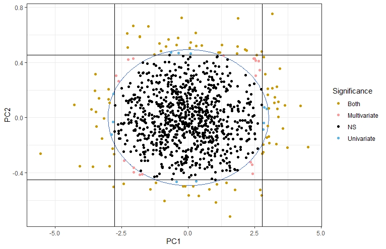
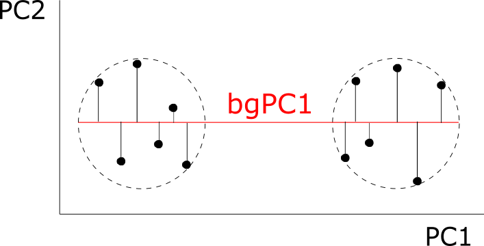
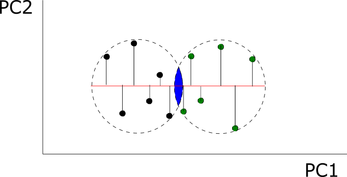
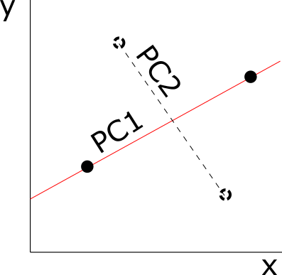
Take 1000 random observations from a bivariate normal distribution where each variable has variance 1 and covariance 0.95. Then, run a PCA for the whole sample and for each observation run a univariate test for each PC and a multivariate test for both variables at the same time. You get four different situations (represented in the figure): a) the observation isn’t significantly different from the rest of the population for any test (in black), b) the observation is significantly different only in its PC1 (in blue, observations off the vertical lines) or PC2 (in blue, observations off the horizontal lines), c) the observation is significantly different only in the multivariate test (in pink, off the blue circle but within the limits of the vertical and horizontal lines), d) significantly different for all tests (in gold, off the circle and the vertical and horizontal lines).

I learned a lot with these simple simulations: I could increase the number of variables, the patterns of covariation, etc. The most valuable lesson I got was that multivariate techniques don’t recover all the statistical signals identified by the univariate methods: multivariate methods are more sensitive in the direction of the covariance (the corners in the figure), while univariate methods detect more often observations in the direction of each axis (aligned with the PCs, as you can see). These conclusions may not be relevant for shape data, where all coordinates are a function of the whole configuration of coordinates (due to the Procrustes superimposition) and that would invalidate theoretically its decomposition in multiple chunks of independent data. Still, an entertaining learning experience.

Edit (4/10/20):

I attach here the original article by Rao, the one nicely explained by Healy (1969) and that are usually cited together. I’m posting it here since I really struggled to find it: I had to visit several libraries in Paris in very particular conditions, which made a funny memory from my postdoc there. Psychologists say that memories are created more easily when the learning experience is coupled with a physical one, maybe that’s why I like this whole thing. Anyway, here you’ve got it:

Rao_paradox Download

(It’s a large file, so it may take few seconds to download)

Three common misunderstandings on modularity and integration

1. Modularity and integration are opposite terms.

This is probably the most common misunderstanding about modularity. We all get integration right: covariation among traits (e. g. among different landmarks placed in a skull). Then, we say: modularity is the statistical independence among subsets of traits. And that’s only partially true. Modularity is the statistical independence among subsets traits *relative to the covariation within each one of them*. We can find two modules with a huge level of covariation within each module and high (but comparatively much lower) covariation between them (i. e. high integration and high modularity). We can also find two modules that show low covariation among modules but also low covariation within modules (low integration and low modularity). So, we can’t just check for integration among modules and conclude from there the existence or not of modularity.

2. Our null hypothesis is that modularity does not exist at all in our structure.

This is the one that gathers the highest number of controversial opinions. For every set of traits (or landmarks) there is always a combination of them (modules) that shows the lowest covariation among them. See for example the principal components, these are axes of variation that are independent (orthogonal) among them. Principal components give you independent modules (ok, not quite because modules need to be adjacent blabla, but you get the idea). There’s always some statistical modularity in your sample (if an appropriate sample size, see previous posts). If you want to cheat yourself, you can just test modularity on the particular subsets showing the least covariation among them and then come up with a biological hypothesis that justifies that pattern (maybe pre-registration would help with that HARKing, controversial opinion 1). So, the important bit of the modularity test is the biological hypothesis tested. Usually you check whether there’s statistical evidence in favor of that particular (and robust) hypothesis, which is true even if you don’t get a significant p-value. In case you don’t have a robust hypothesis a priori, that’s also good news: you may propose one based on the morphological pattern of your sample. But, for that, you don’t need hypothesis testing and a p-value, you just need to do descriptive statistics (showing the modularity pattern of your sample), which is as interesting as hypothesis testing (controversial opinion 2).

3. We only care about modularity and integration if we’re interested in modularity and integration.

I’ll be very brief here. Andrea Cardini and others (I don’t have the ref in hand, but there’s a paper) have shown that Procrustes superimposition increases covariation among landmarks. The translation of the Procrustes coordinates into a tangent space may also artificially transform the patterns of covariation (C. Klingenberg showed that in an oral presentation). So, you’re transforming your patterns of covariation (integration and modularity) just with the superimposition, despite whether these features are of your interest or not.

My two cents on the between-group PCA issue

Some weeks ago F. Bookstein announced in morphmet his last paper, in which he warned about an artifactual separation between groups when we use a between-group PCA. Following that message there were many others, some related to authorship issues (which I won’t comment) and some others related to technical ones.

So first, what’s a between-group PCA? A between-group PCA is one kind of discriminant analysis where you maximize the separation among pre-defined groups. To do that, we first run a PCA on the group means and then individuals are projected on the axes of that group-means PCA. Because it’s based on a rotation of the original space (PCA) and not on the estimation of variance and a subsequent deformation of the space (e. g. CVA) it’s considered robust against data with high dimensionality/sample sizes ratios (here you may be interested in reading my first post on PCA and dimensionality).

Imagine one population (black), where you run a PCA so you get a visualization like this (PC1 & PC2). If you make two groups out of your population (dashed circles) and you run a PCA on the means you will get just one axis (bgPC1, N-1) , that connects the centre of each circle. Finally, each individual would be projected on this new axis to get the between-group PCA scores.

So the problem people have noticed is that as the dimensionality exceeds the sample size, the between-group PCA strongly differentiates the groups we ask to discriminate no matter how arbitrary they are. It makes sense: when we run a PCA on the group means we highly reduce the dimensionality to N-1 dimensions (where N is the number of groups). Then, the projection of each individual to these few dimensions reduces the variance within groups (as in my beloved Albrecht 1980 figure but reading it from the bivariate plot to the two univariate plots):

Imagine the same situation as in figure 1 but with some overlap between the groups (blue area). This area of overlap is indeed larger in two-dimensions (blue area) than in one dimension (red line within blue area). As we increase the dimensionality, the area of overlap in one dimension becomes smaller in relation to the original area of overlap (volume of two spheres in 3D, hypervolume of two hyperspheres for more than 3 dimensions). Separation among groups will be larger and larger.

Now, Philip Mitteroecker also pointed out an interesting fact: even when we use a high number of landmarks, we find covariation (integration) among variables and therefore effective dimensionality is never going to be really high. Therefore, ‘many of the problems described by Cardini et al. and Fred can be avoided by variable reduction (ordinary PCA) prior to bgPCA and related techniques’.

That is only true if, pay attention, the pattern of covariation within groups is similar to the pattern of covariation among groups. When both patterns are equal, then the PCA on the raw sample will be equivalent to the between-group PCA and therefore no artefacts show up. When within-groups variation is perpendicular to the among group variation, then we’ll find a collapse of the within-group variance. Actually, on the extreme, this second situation would be analogous to run a PCA on the group means and then place the individuals on their group centroid:

Two examples of between-group PCA with anisotropic variation. In the first case, the one I think Philip Mitteroecker had in mind and probably the most likely when the two groups are evolutionary close, the major axis of variation within-group is the same than the axis of variation among groups. On the extreme, within-group variation could be two straight lines overlapping with the bgPC1 (red line): in that situation the original disposition of the individuals would be equivalent to the distribution after the between group-PCA.
In the second case, however, within-group variation is perpendicular to among-group variation. On the extreme, within-group would be represented by two lines perpendicular to the bgPC1 (red line). In that situation the projection of the individuals on the new axis would completely remove within-group variation and it would also reduce (but comparatively much less) variation among individuals from the two groups.

While it’s certainly true that in the first case anisotropic variation reduces the problem of spurious separation of groups (because population PCA and bgPCA would be equivalent), the second case would make it much worse. When population grouping is based on, for example, on evolutionary relatedness, it is unlikely that within-group variation will be perpendicular to among-group variation. However, for some other kind of groups (e. g. response to one environmental factor) that might happen.

Here’s my two cents on the between-group PCA issue.

CVG

On the dimensionality in morphometrics

High-dimensional and Multivariate stuff

Few years ago I started to read and listen that shape is a high-dimensional AND multivariate character (e. g. in Klingenberg & Gidazewski Sys Bio 2010 or in a talk by Dean Adams at the SMEF 16 in Paris). To my embarrassment it wasn’t until some time afterwards that I understood why these adjectives weren’t synonyms. Shape is usually described by a large set of variables or measurements, which makes it high-dimensional, but these variables need to be considered altogether when analyzed statistically, which makes shape multivariate. The alternative would be to assess variation on each variable independently, but that would be less efficient (you would lose track of covariation among variables, to visualize that I love the figure in Albretch Am Zool 1980). Also, the multiple univariate assessment of shape variables would be conceptually incorrect for geometric morphometrics (what’s the meaning of one or few landmarks when the superimposition was run for all of them?).

Curse of the dimensionality

So shape analyses consist on the variation of many variables on many individuals, all at the same time. Intuitively, we could think that the more variables the better: a more accurate description of the individual shape would maximize the differences among the individuals and therefore obtain the important features in the sample shape variability. Graphical representations would have more resolution too.

Now, the question is how many individuals per variable. Is that important? Let’s use a toy example with two individuals and two variables. Imagine we were interested in looking at the association between these two shape variables in our sample of 2 individuals:

So: imagine we want to test an association between two shape variables x and y and two individuals. Know what? Always a perfect association.

There are two ways of thinking at this. One I borrow from Chris Klingenberg: you will always find a perfect association between two variables with just two individuals because you can always find a straight line connecting two points. From a different perspective : to *fairly* test for an association between variables, you need a sample size that allows you *not* to find an association. That means a sample size that could show equal variation in all the directions of the bidimensional space (i. e. draw a circumference).

With two more individuals would be enough not to find an association between variables. *If these new individuals were perpendicular to the association between the first two,* the association represented by the red line wouldn’t be more likely than any other association. Ok, just four ind. might still not be ideal, but at least we aren’t sure about the result in advance.

Ok, maybe you’re not interested in testing the association among shape variables. But what about a PCA? Everybody has done a PCA on shape variables. Haven’t you realized that the number of PCs obtained are either 2k-4 for 2D datasets (k = number of landmarks, 3k-7 for 3D datasets) or N-1 (N number of individuals)? That depends on the number of individuals per variable. The PCA is an ordination method where orthogonal axes of variation are estimated: as in our toy example, the number of axes of variation will depend on the individuals per variable. In the case of two individuals and two variables, there is just one axis of variation, so one PC (N-1 PCs). If we add more individuals then a second axis of variation will show up and then we’ll get two PCs (2k-4 for 2D landmark data).

In our first figure (just 2 ind.) we would find just one axis of variation (PC1), so the number of PCs = N-1. With two more ind. we would add a second PC, so the number of PCs = number of variables. In GMM, to the total number of variables we remove 4 (2D) or 7 (3D) because of the superimposition.

It makes sense, doesn’t it? With a PCA we remove all the directions of the phenotypic space in which there isn’t evidence of variation and we just keep the least possible variation per variable (i. e. only the variation differentiating our individuals), a line for two variables, a plane for three, etc. Actually, we sort of do that in our daily life: if I start to talk about my group of friends I will probably give you the least amount of information needed to differentiate each one of them, even though each one is different from the rest in millions of ways.

This has important consequences: first, that some of the variation we have theoretically considered with the addition of each variable is removed afterwards. If we run subsequent analyses on our PCs, we will not consider this theoretical variation. In addition, for certain statistical analyses (as covariation tests) we will always have an over-estimation of our estimates if our sample size is smaller or similar to our number of variables (remember? Always a perfect line between two points no matter the dimensionality).

Related to that, using more variables than individuals there will always be a combination of variables separating no matter which group of individuals we’re interested in (a problem leading to overfitting in regression and machine learning techniques): try to describe two people with two parameters (x and y), which can take values either 0 or 1. Only rule: both parameters can’t take the same values for both people (that wouldn’t count as 2 parameters). Spoiler: (at least) one of the parameters will be different for each person (so yes, for 2 individuals in 2D there’s just one PC with all the variance).

CVG