Blog

I’m not rejecting articles

Just a brief note on something (one more thing) I don’t understand about academic publishing.

Nobody has ever explained to me in detail what a journal expects from me as a reviewer. Nobody has explained to me what a review exactly must be. I just pretend to go along with a tradition everybody seems to know fairly well although it’s clear nobody really does. This sounds pretty absurd but it’s quite common in academia.

The blurred idea we all have about peer-review is that few colleagues with a fair knowledge of your subject of interest give some unreplicable (so, statistically speaking, random) opinions about your work so that you can improve it (hopefully) and they can help the editors to decide whether your article is good enough to be published in their journal.

This last bit is the one that bugs me: I’m sorry, I can’t say whether an article is good/important enough for the standards of your journal. I don’t think it’s fair that professional careers depend at some extend on my arbitrary opinion as a reviewer (since we all care so much about individual publication records) and I won’t damage anybody (even if it’s only a little bit) based on my particular taste. And even if I’m sure I’m right, I don’t want to act as a gatekeeper: I want different perspectives to be included, not only those I like.

That doesn’t change the fact that you can be exigent: if there’s something false, you can say you think it’s false. If conclusions can’t be deduced from the results, you can also say so. But that doesn’t change the fact that 1) maybe you’re wrong, 2) authors could always change what you think it’s wrong or incomplete, 3) maybe the article is valuable for some other reason. And even if you think the article is horrible, remember it is probably going to be published elsewhere anyway.

Then, yes, controversial articles may be considered at the same level than more robust articles, but isn’t it the case already? And for that I blame the fact that the journals don’t publish the reviews along with the articles (which makes the review process less transparent and brings all the known problems opaque procedures are known for).

So, my policy as a reviewer is: accepting to review only for society journals or non-profit organizations, writing lengthy reviews that give as much information as possible to the authors and finally, unless there’s something grossly wrong (i. e. the suspicion of some dishonest behaviour), I’m accepting the article.

Multivariate analysis vs multiple univariate analyses

I once read a paper where the author said that shape’s a multidimensional and multivariate character. That let me thinking for months on the difference between these two terms. The next summer, during an oral presentation, a different scientist repeated that same sentence, this time explaining that shape’s a multidimensional character due to the number of variables that are used to describe it and a multivariate character due to the statistical treatment this character must receive to be analysed. Contrary to univariate analyses, multivariate techniques take into account multiple variables at the same time, meaning that they consider the correlation among variables (although they often assume the independence among them). Once we have many variables describing a phenotype, we can either apply one multivariate method to analyze this phenotype all at once or we can apply multiple univariate methods to decompose this phenotype in unrelated chunks of data.

As far as I’ve read, over the last 60 years there was a controversy in the scientific literature about which approach was optimal on the analyses of multidimensional data. Today, the vast majority of scientists (at least in geometric morphometrics) consider multivariate methods the standard, the most powerful approach to analyze shape data. However, not so long ago I read a paper that stroke me for its simplicity and how well it explained the difficult relationship between multivariate and univariate approaches: Healy (1969) (I hope you didn’t expect a recent paper).

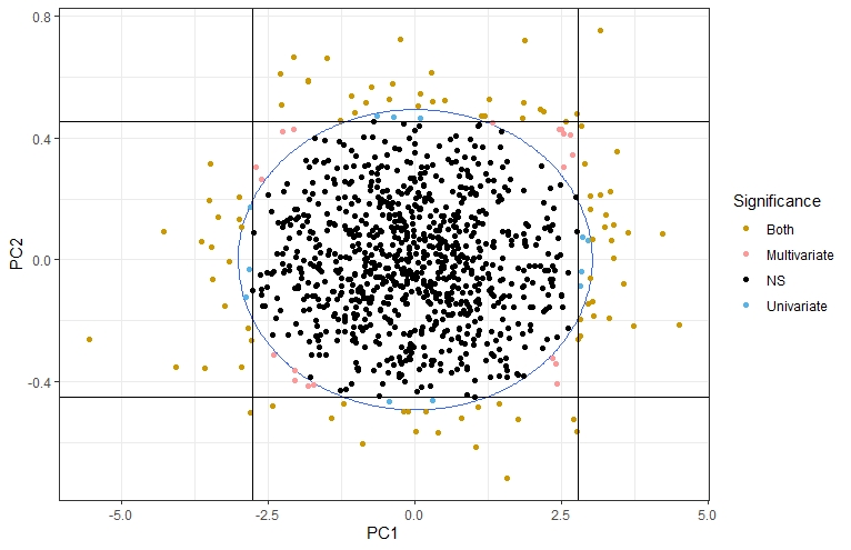
I liked it so much that I replicated the figure showing the whole argument:

Take 1000 random observations from a bivariate normal distribution where each variable has variance 1 and covariance 0.95. Then, run a PCA for the whole sample and for each observation run a univariate test for each PC and a multivariate test for both variables at the same time. You get four different situations (represented in the figure): a) the observation isn’t significantly different from the rest of the population for any test (in black), b) the observation is significantly different only in its PC1 (in blue, observations off the vertical lines) or PC2 (in blue, observations off the horizontal lines), c) the observation is significantly different only in the multivariate test (in pink, off the blue circle but within the limits of the vertical and horizontal lines), d) significantly different for all tests (in gold, off the circle and the vertical and horizontal lines).

I learned a lot with these simple simulations: I could increase the number of variables, the patterns of covariation, etc. The most valuable lesson I got was that multivariate techniques don’t recover all the statistical signals identified by the univariate methods: multivariate methods are more sensitive in the direction of the covariance (the corners in the figure), while univariate methods detect more often observations in the direction of each axis (aligned with the PCs, as you can see). These conclusions may not be relevant for shape data, where all coordinates are a function of the whole configuration of coordinates (due to the Procrustes superimposition) and that would invalidate theoretically its decomposition in multiple chunks of independent data. Still, an entertaining learning experience.

Edit (4/10/20):

I attach here the original article by Rao, the one nicely explained by Healy (1969) and that are usually cited together. I’m posting it here since I really struggled to find it: I had to visit several libraries in Paris in very particular conditions, which made a funny memory from my postdoc there. Psychologists say that memories are created more easily when the learning experience is coupled with a physical one, maybe that’s why I like this whole thing. Anyway, here you’ve got it:

(It’s a large file, so it may take few seconds to download)

Mathematicians vs Computer scientists

Lately, I’ve started to learn some machine learning. As an intro, I’ve completed one of the coursera MOOCs devoted to that, in particular the Machine Learning course designed by Stanford University. I find MOOCs super useful introductory courses. It was a nice experience and I learnt many things I didn’t expect to learn. In first place: Octave. As Blas Benito told me on Twitter, Octave is a fully-developed programming language ‘compatible’ with Matlab (I grossly labelled it as a ‘open-source version of Matlab’). I worked a bit with Matlab during my PhD but then I abandoned all my scripts because it isn’t free, I wish I had known back then Octave. Anyway, the whole Machine Learning course is developed with scripts and exercises in Octave (which is quite intuitive if you already know R).

Now, to better integrate the exercises and just in case I want to use some of the methods in my future research, I’ve translated all the exercises and scripts to R. You can find them in my Gitlab site. Over the next few weeks I hope I’ll get to translate them to Python too, as this could help me to catch-up with Python. In the near future I’d also like to develop these scripts to accommodate multivariate data as dependent values (maybe at the same time I write the Python functions).

One of the things that really got my attention during this course was the first lesson, on linear regression. I already knew how to run a linear regression from scratch and to estimate analytically the least-squares linear function, with its slope and intercept. When I saw they were explaining an iterative process to obtain the best-fitting linear function I got the impression that they were using an unnecessary complicated process based on brute-force principles to estimate something pretty simple. When things got complicated later, I understood that this was a necessary introduction for more complex cases.

I still think mathematicians and statisticians would be puzzled by the long procedures used by data scientists, while computer scientists might be amazed by the efficiency of such a long array of algorithms ran on high-dimensional data. At the same time, I don’t think mathematicians and statisticians have a clear answer for many of the questions where high-dimensional data is involved while computer scientists, even if by unsophisticated means, have found their way into largely unexplored areas with reasonable efficiency. Maybe trying to figure out an analytical way of explaining the algorithmic results would be the golden ticket. Meanwhile, I’ll stick to algorithms whenever I need them but there’s no way I’ll abandon normal equations for linear regression.

Three common misunderstandings on modularity and integration

1. Modularity and integration are opposite terms.

This is probably the most common misunderstanding about modularity. We all get integration right: covariation among traits (e. g. among different landmarks placed in a skull). Then, we say: modularity is the statistical independence among subsets of traits. And that’s only partially true. Modularity is the statistical independence among subsets traits *relative to the covariation within each one of them*. We can find two modules with a huge level of covariation within each module and high (but comparatively much lower) covariation between them (i. e. high integration and high modularity). We can also find two modules that show low covariation among modules but also low covariation within modules (low integration and low modularity). So, we can’t just check for integration among modules and conclude from there the existence or not of modularity.

2. Our null hypothesis is that modularity does not exist at all in our structure.

This is the one that gathers the highest number of controversial opinions. For every set of traits (or landmarks) there is always a combination of them (modules) that shows the lowest covariation among them. See for example the principal components, these are axes of variation that are independent (orthogonal) among them. Principal components give you independent modules (ok, not quite because modules need to be adjacent blabla, but you get the idea). There’s always some statistical modularity in your sample (if an appropriate sample size, see previous posts). If you want to cheat yourself, you can just test modularity on the particular subsets showing the least covariation among them and then come up with a biological hypothesis that justifies that pattern (maybe pre-registration would help with that HARKing, controversial opinion 1). So, the important bit of the modularity test is the biological hypothesis tested. Usually you check whether there’s statistical evidence in favor of that particular (and robust) hypothesis, which is true even if you don’t get a significant p-value. In case you don’t have a robust hypothesis a priori, that’s also good news: you may propose one based on the morphological pattern of your sample. But, for that, you don’t need hypothesis testing and a p-value, you just need to do descriptive statistics (showing the modularity pattern of your sample), which is as interesting as hypothesis testing (controversial opinion 2).

3. We only care about modularity and integration if we’re interested in modularity and integration.

I’ll be very brief here. Andrea Cardini and others (I don’t have the ref in hand, but there’s a paper) have shown that Procrustes superimposition increases covariation among landmarks. The translation of the Procrustes coordinates into a tangent space may also artificially transform the patterns of covariation (C. Klingenberg showed that in an oral presentation). So, you’re transforming your patterns of covariation (integration and modularity) just with the superimposition, despite whether these features are of your interest or not.

Memories and delusions on phylogenetic comparative methods in econometrics

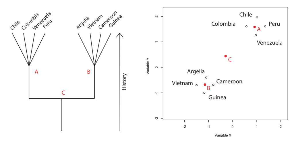
Today, navigating among the old files in my computer, I found a text and some figures in which I tried to explain why comparative methods might be of interest for people studying macroeconomy. I just applied the same reasoning we usually do in biology: countries are not independent entities since historically they’ve had different degrees of relationships (some have arisen from some others). Therefore, the type of relationship among macroeconomic variables we usually see in graphs with a large number of countries might only reflect a random correlation product of the historical relationship among countries. I know, this kind of metaphors biology-economy (or evolution-history) are flawed and, as one of my former bosses put it once: ‘the danger of metaphors is that the better they are the less they look like a metaphor’.

That’s probably why it was among old files in my computer, where this kind of fast idea should be, and I’m happy to say that. However, because this blog is a bit of a jumble too, I thought I’d share the graphs here:

Here, ‘Felsenstein’s best case scenario’
Here, ‘Felsenstein’s worst case scenario’

Estoy escribiendo un libro de estadística multivariante

Lo he repetido sin parar en los últimos meses. Me digo que así sentiré la presión de terminar por fin un pequeño proyecto que tengo aparcado desde hace tres o cuatro años, aunque sea por la vergüenza de pensar que quizá alguien me pregunte en un futuro que dónde está.

Bueno, en realidad no es un libro LIBRO. Es más bien un pequeño manual. Bueno, más bien un manual para mí mismo, pero entiendo que puede servir para otros. Me dije que podría redactar un pequeño manual de consulta con todos los pormenores de las técnicas de estadística multivariante que más utilizo (usadas en morfometría, vaya). Aquí os dejo el índice:

  • Introducción
  • Vectores y matrices: propiedades y operaciones
  • Estadística descriptiva: media y matriz de covarianza, espacios, distancias y correlaciones
  • Reorganización de datos: Análisis de componentes principales, escalado multidimensional, mínimos cuadrados parciales, análisis discriminantes, clustering
  • Normalidad: MANOVA, Regresión lineal múltiple y multivariante
  • Bootstrap y permutaciones

Si falta algo me decís.

Mi idea es, para cada concepto:

  • Pequeña introducción sobre lo que es y para qué se suele usar
  • Mostrar el desarrollo analítico (a mano vaya, como en el cole) junto con un ejemplo numérico para dos variables
  • Visualización para dos variables
  • Comentar lo que ocurre cuando el número de variables aumenta y en particular cuando el número de variables es mayor que el número de sujetos
  • Adjuntar un script R con su estimación usando sólo funciones lo más básicas posibles

Mi primera idea fue subirlo aquí una vez que lo termine y que se lo baje quien quiera, por aquello del open-access, el bien común, y otros conceptos hippies que me atraen. Después pensé que prefiero publicarlo con alguna editorial (si encuentro alguna) porque me gustaría que el manuscrito pasara un proceso de edición. En fin, cuando lo esté terminando (en unas semanas, espero) veré. En todo caso a quien me lo pida personalmente se lo pasaré.

Habrá para todos, no empecéis a saquear las librerías todavía.

CVG

Summer reads (papers)

Over the last few weeks of holidays I’ve started to store some papers I’d like to read. Now I’ve got all my devices and apps full of references, open and with no particular order, which is causing me a bit of stress (obsessive-compulsive disorder alert). I thought it may be useful to write a post with all the references so that they’re out of my daily activities and I can find all of them fast in few days. Plus, they may be interesting for other people. Here they are:

Inherent forms and the evolution of evolution (S. A. Newman):

John Bonner presented a provocative conjecture that the means by which organisms evolve has itself evolved. The elements of his postulated nonuniformitarianism in the essay under discussion—the emergence of sex, the enhanced selection pressures on larger multicellular forms—center on a presumed close mapping of genotypic to phenotypic change. A different view emerges from delving into earlier work of Bonner’s in which he proposed the concept of “neutral phenotypes” and “neutral morphologies” allied to D’Arcy Thompson’s analysis of physical determinants of form and studied the conditional elicitation of intrinsic organizational properties of cell aggregates in social amoebae. By comparing the shared and disparate mechanistic bases of morphogenesis and developmental outcomes in the embryos of metazoans (animals), closely related nonmetazoan holozoans, more distantly related dictyostelids, and very distantly related volvocine algae, I conclude, in agreement with Bonner’s earlier proposals, that understanding the evolution of multicellular evolution requires knowledge of the inherent forms of diversifying lineages, and that the relevant causative factors extend beyond genes and adaptation to the physics of materials.

Making and breaking symmetry in development, growth and disease (D. T. Grimes):

Consistent asymmetries between the left and right sides of animal bodies are common. For example, the internal organs of vertebrates are left-right (L-R) asymmetric in a stereotyped fashion. Other structures, such as the skeleton and muscles, are largely symmetric. This Review considers how symmetries and asymmetries form alongside each other within the embryo, and how they are then maintained during growth. I describe how asymmetric signals are generated in the embryo. Using the limbs and somites as major examples, I then address mechanisms for protecting symmetrically forming tissues from asymmetrically acting signals. These examples reveal that symmetry should not be considered as an inherent background state, but instead must be actively maintained throughout multiple phases of embryonic patterning and organismal growth.

Genomics of developmental plasticity in animals (E. Lafuente & P. Beldade):

Developmental plasticity refers to the property by which the same genotype produces distinct phenotypes depending on the environmental conditions under which development takes place. By allowing organisms to produce phenotypes adjusted to the conditions that adults will experience, developmental plasticity can provide the means to cope with environmental heterogeneity. Developmental plasticity can be adaptive and its evolution can be shaped by natural selection. It has also been suggested that developmental plasticity can facilitate adaptation and promote diversification. Here, we summarize current knowledge on the evolution of plasticity and on the impact of plasticity on adaptive evolution, and we identify recent advances and important open questions about the genomics of developmental plasticity in animals. We give special attention to studies using transcriptomics to identify genes whose expression changes across developmental environments and studies using genetic mapping to identify loci that contribute to variation in plasticity and can fuel its evolution.

The evolution of phenotypic correlations and ‘developmental memory’ (R. A. Watson, G. P. Wagner, M. Pavlicev, D. W. Weinrich, R. Mills):

Development introduces structured correlations among traits that may constrain or bias the distribution of phenotypes produced. Moreover, when suitable heritable variation exists, natural selection may alter such constraints and correlations, affecting the phenotypic variation available to subsequent selection. However, exactly how the distribution of phenotypes produced by complex developmental systems can be shaped by past selective environments is poorly understood. Here we investigate the evolution of a network of recurrent nonlinear ontogenetic interactions, such as a gene regulation network, in various selective scenarios. We find that evolved networks of this type can exhibit several phenomena that are familiar in cognitive learning systems. These include formation of a distributed associative memory that can “store” and “recall” multiple phenotypes that have been selected in the past, recreate complete adult phenotypic patterns accurately from partial or corrupted embryonic phenotypes, and “generalize” (by exploiting evolved developmental modules) to produce new combinations of phenotypic features. We show that these surprising behaviors follow from an equivalence between the action of natural selection on phenotypic correlations and associative learning, well‐understood in the context of neural networks. This helps to explain how development facilitates the evolution of high‐fitness phenotypes and how this ability changes over evolutionary time.

Evolutionary significance of phenotypic accommodation in novel environments: an empirical test of the Baldwin effect (A. V. Badyaev):

When faced with changing environments, organisms rapidly mount physiological and behavioural responses, accommodating new environmental inputs in their functioning. The ubiquity of this process contrasts with our ignorance of its evolutionary significance: whereas within-generation accommodation of novel external inputs has clear fitness consequences, current evolutionary theory cannot easily link functional importance and inheritance of novel accommodations. One hundred and twelve years ago, J. M. Baldwin, H. F. Osborn and C. L. Morgan proposed a process (later termed the Baldwin effect) by which non-heritable developmental accommodation of novel inputs, which makes an organism fit in its current environment, can become internalized in a lineage and affect the course of evolution. The defining features of this process are initial overproduction of random (with respect to fitness) developmental variation, followed by within-generation accommodation of a subset of this variation by developmental or functional systems (‘organic selection’), ensuring the organism’s fit and survival. Subsequent natural selection sorts among resultant developmental variants, which, if recurrent and consistently favoured, can be inherited when existing genetic variance includes developmental components of individual modifications or when the ability to accommodate novel inputs is itself heritable. Here, I show that this process is consistent with the origin of novel adaptations during colonization of North America by the house finch. The induction of developmental variation by novel environments of this species’s expanding range was followed by homeostatic channelling, phenotypic accommodation and directional cross-generational transfer of a subset of induced developmental outcomes favoured by natural selection. These results emphasize three principal points. First, contemporary novel adaptations result mostly from reorganization of existing structures that shape newly expressed variation, giving natural selection an appearance of a creative force. Second, evolutionary innovations and maintenance of adaptations are different processes. Third, both the Baldwin and parental effects are probably a transient state in an evolutionary cycle connecting initial phenotypic retention of adaptive changes and their eventual genetic determination and, thus, the origin of adaptation and evolutionary change.

Bonus tracks:

Why the reward structure of science makes reproducibility problems inevitable? (R. Heesen):

Recent philosophical work has praised the reward structure of science, while recent empirical work has shown that many scientific results may not be reproducible. I argue that the reward structure of science incentivizes scientists to focus on speed and impact at the expense of the reproducibility of their work, thus contributing to the so-called reproducibility crisis. I use a rational choice model to identify a set of sufficient conditions for this problem to arise, and I argue that these conditions plausibly apply to a wide range of research situations. Currently proposed solutions will not fully address this problem. Philosophical commentators should temper their optimism about the reward structure of science.

Null hypothesis significance testing: A review of an old and continuing controversy (R. S. Nickerson):

Null hypothesis significance testing (NHST) is arguably the most widely used
approach to hypothesis evaluation among behavioral and social scientists. It is also
very controversial. A major concern expressed by critics is that such testing is
misunderstood by many of those who use it. Several other objections to its use have
also been raised. In this article the author reviews and comments on the claimed
misunderstandings as well as on other criticisms of the approach, and he notes
arguments that have been advanced in support of NHST. Alternatives and supplements to NHST are considered, as are several related recommendations regarding
the interpretation of experimental data. The concluding opinion is that NHST is
easily misunderstood and misused but that when applied with good judgment it can
be an effective aid to the interpretation of experimental data.

CVG
Two-speed academia

I’m in Providence since last Thursday, attending the Evolution meeting. One of the main talks was dedicated to mention some possible sources of error when conducting research and to advocate for open science and replicable methods.

I fully agree with the need for replicability and open science to improve the quality of research. Indeed, during my last postdoc I’ve started myself to dedicate much more time to comment R scripts, write reports in markdown to explain my methods… etc. Maybe that’s why when I listened to the different habits we should develop when conducting research I thought: ‘what an extra load of work’.

Does it matter? Is it really important to finish up your paper 6 months before or later? Well, if you’ve got a permanent position it may not. If you’ve got a 3-year PhD scholarship or a 1-year postdoc contract it does, a lot.

Since some time ago I’ve realized that there’s a clear separation between the work of permanent researchers and the work of PhD students and postdocs. I think it’s clearly associated with the contrast between the stability of permanent positions and the wild competition in the job market (with publication records, impact factors and other bullshit). We’re in a two-speed academia, where permanent researchers are ‘running for their dinner’ and temporal researchers ‘running for their lives’.

Should we care about this? Should we stop improving science because our society is unfair? Well, the same way it isn’t ethical to care only about the career of temporal researchers despising research quality (i. e. publishing a lot, no matter what), I don’t think it’s right to ask them to work more and harder while carrying on with this mad system (i. e. sentencing the young authors of some wonderful work to unemployment). In other words, I think science has bigger problems than the lack of open science and maybe even related to it: if we improve the work conditions of the young researchers (the main workforce), we will probably improve the work quality in science.

Here an example:

CVG.

My two cents on the between-group PCA issue

Some weeks ago F. Bookstein announced in morphmet his last paper, in which he warned about an artifactual separation between groups when we use a between-group PCA. Following that message there were many others, some related to authorship issues (which I won’t comment) and some others related to technical ones.

So first, what’s a between-group PCA? A between-group PCA is one kind of discriminant analysis where you maximize the separation among pre-defined groups. To do that, we first run a PCA on the group means and then individuals are projected on the axes of that group-means PCA. Because it’s based on a rotation of the original space (PCA) and not on the estimation of variance and a subsequent deformation of the space (e. g. CVA) it’s considered robust against data with high dimensionality/sample sizes ratios (here you may be interested in reading my first post on PCA and dimensionality).

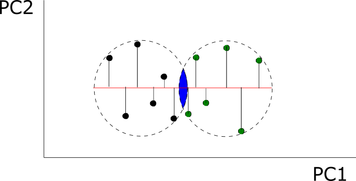
Imagine one population (black), where you run a PCA so you get a visualization like this (PC1 & PC2). If you make two groups out of your population (dashed circles) and you run a PCA on the means you will get just one axis (bgPC1, N-1) , that connects the centre of each circle. Finally, each individual would be projected on this new axis to get the between-group PCA scores.

So the problem people have noticed is that as the dimensionality exceeds the sample size, the between-group PCA strongly differentiates the groups we ask to discriminate no matter how arbitrary they are. It makes sense: when we run a PCA on the group means we highly reduce the dimensionality to N-1 dimensions (where N is the number of groups). Then, the projection of each individual to these few dimensions reduces the variance within groups (as in my beloved Albrecht 1980 figure but reading it from the bivariate plot to the two univariate plots):

Imagine the same situation as in figure 1 but with some overlap between the groups (blue area). This area of overlap is indeed larger in two-dimensions (blue area) than in one dimension (red line within blue area). As we increase the dimensionality, the area of overlap in one dimension becomes smaller in relation to the original area of overlap (volume of two spheres in 3D, hypervolume of two hyperspheres for more than 3 dimensions). Separation among groups will be larger and larger.

Now, Philip Mitteroecker also pointed out an interesting fact: even when we use a high number of landmarks, we find covariation (integration) among variables and therefore effective dimensionality is never going to be really high. Therefore, ‘many of the problems described by Cardini et al. and Fred can be avoided by variable reduction (ordinary PCA) prior to bgPCA and related techniques’.

That is only true if, pay attention, the pattern of covariation within groups is similar to the pattern of covariation among groups. When both patterns are equal, then the PCA on the raw sample will be equivalent to the between-group PCA and therefore no artefacts show up. When within-groups variation is perpendicular to the among group variation, then we’ll find a collapse of the within-group variance. Actually, on the extreme, this second situation would be analogous to run a PCA on the group means and then place the individuals on their group centroid:

Two examples of between-group PCA with anisotropic variation. In the first case, the one I think Philip Mitteroecker had in mind and probably the most likely when the two groups are evolutionary close, the major axis of variation within-group is the same than the axis of variation among groups. On the extreme, within-group variation could be two straight lines overlapping with the bgPC1 (red line): in that situation the original disposition of the individuals would be equivalent to the distribution after the between group-PCA.
In the second case, however, within-group variation is perpendicular to among-group variation. On the extreme, within-group would be represented by two lines perpendicular to the bgPC1 (red line). In that situation the projection of the individuals on the new axis would completely remove within-group variation and it would also reduce (but comparatively much less) variation among individuals from the two groups.

While it’s certainly true that in the first case anisotropic variation reduces the problem of spurious separation of groups (because population PCA and bgPCA would be equivalent), the second case would make it much worse. When population grouping is based on, for example, on evolutionary relatedness, it is unlikely that within-group variation will be perpendicular to among-group variation. However, for some other kind of groups (e. g. response to one environmental factor) that might happen.

Here’s my two cents on the between-group PCA issue.

CVG

Los p-valores y el procés

Twitter me ha dado una excusa magnífica para explicar un fenómeno de moda en mi trabajo y no pienso dejarla escapar. En realidad, este fenómeno va más allá de mi trabajo: es un concepto estadístico y está últimamente en boca de todo el mundo en ciencias y ciencias sociales (sobre todo para mal). Son los p-valores. Aprovecho para contarlo en versión técnica y en versión ‘juicio del procés’.

Versión técnica:

Imaginad que queréis saber si el nuevo medicamento para bajar la tensión que habéis desarrollado funciona o no. ¿Qué hacemos? Pues hacemos dos grupos de personas: un grupo toma el medicamento y el otro no. Entonces, les medimos la tensión a las personas de los dos grupos y vemos si hay diferencia entre las medias de los grupos. Si el grupo al que le hemos dado el medicamento tiene la tensión más baja que el grupo control, quizá nuestro medicamento esté funcionando.

¿Solamente ‘quizá’? Solamente quizá, porque si la diferencia entre los dos grupos es mínima a lo mejor la diferencia no es por el medicamento sino por mil otras cosas que pueden estar influyendo de manera diferente a los dos grupos por azar. Entonces hacemos un pequeño cálculo: Si suponemos que la tensión varía de manera aleatoria entre los individuos de la población, ¿cuál es la probabilidad de obtener una diferencia entre dos grupos de personas al azar como la que hemos obtenido o más grande? Esa probabilidad es un p-valor. Cuanto más bajo sea, más sugiere que la diferencia entre nuestro grupo control y el grupo que ha tomado el medicamento no es debido al azar. ¿Cuál es el debate? Mira, os lo voy a explicar con el procés.

Versión procés:

Encuentro este artículo en Twitter, escrito por un señor con muchos seguidores. Habla sobre el juicio del procés, lo titula ‘Cuando una moneda siempre cae del mismo lado’ y en el texto incluye ese parrafito que veis. ¿Se parece a lo que acabo de explicar, verdad? Cuando un p-valor es muy bajo, cuando la probabilidad de que algo haya ocurrido al azar es muy baja, debe de haber un mecanismo de interés por detrás que lo está afectando.

Pues el p-valor está últimamente muy criticado y os ilustro por qué con este párrafo:

  1. ¿Qué es ‘sistemáticamente’? ¿Tirar la moneda 2 veces? ¿4? ¿50? Además, que la probabilidad sea baja no quiere decir que sea nula: se puede tirar una moneda al aire 6 veces y que las 6 veces te salga cruz. Es difícil, pero no imposible. Que una cosa sea improbable no es una garantía de nada: a todos nos pasan cosas improbables continuamente.
  2. ¿Te sorprendería si en vez de una moneda fuera un dado? ¿Te sorprendería tirar un dado 6 veces y que ninguna te saliera un tres? A mí no mucho. ¿Por qué comparamos esta situación con una moneda y no con un dado? ¿A lo mejor habría que pensar mejor las condiciones con las que describimos ‘el azar’? Porque si no, estamos manipulando.
  3. ¿’La probabilidad de que alguien esté dirigiendo la moneda‘? Las monedas no son perfectas: están deformadas, no son regulares en su peso… A la larga, una moneda va a caer sistemáticamente de un lado por su propias imperfecciones, no necesito a nadie dirigiendo la moneda. De hecho: ¿cómo se ‘dirige’ una moneda? La estadística te puede dar una probabilidad, pero no la interpreta: cuando este señor se encuentra una moneda que siempre cae del mismo lado él piensa que hay alguien trucando las tiradas y yo diría que es simplemente una moneda deformada.

Así que los p-valores son herramientas, si se utilizan bien, para ver cuándo algo sale de la normalidad. Si eso es relevante (o no) es otra cosa y hay que explicarlo bien. No podemos usar una probabilidad como una garantía de que las cosas pasen como nosotros decimos.

De hecho, la desafortunada metáfora de este periodista sólo mostraría que el transcurso del juicio seguramente no ha sido resultado del azar. Pues eso esperábamos todos; la verdad.

CVG